In this tutorial, we are going to learn how to plot Candles and the Simple Moving Average (SMA) technical indicator in Rust. We will use the plotters crate to make drawing a plot or chart easy. This will be a quick tutorial to learn the basics. For this simple tutorial, the data we will use is hard-coded data. In the next tutorial, we will download data from a real source and plot other technical indicators too.
To calculate the Simple Moving Average we will use a function we wrote in an earlier tutorial: How to: technical indicators with Rust and Binance. Please refer to that tutorial for more details on how the SMA algorithm works.
The complete project code can be found on my GitHub: https://github.com/tmsdev82/rust-plotters-sma-tutorial.
Contents
Prerequisites
Some Rust programming knowledge is certainly helpful. Though I explain a number of things, I don’t talk about the Rust basics very much.
Project set up
First, let’s create the “plot SMA using rust” project using cargo: cargo new rust-plotters-sma-tutorial.
The next step is adding the dependencies we need to complete this project:
[package]
name = "rust-plotters-sma-tutorial"
version = "0.1.0"
edition = "2021"

# See more keys and their definitions at https://doc.rust-lang.org/cargo/reference/manifest.html

[dependencies]
chrono = "0.4.19"
plotters = "0.3.1"
We are only using two dependencies:
- chrono:Date and time library for Rust.
- plotters: A Rust drawing library focus on data plotting for both WASM and native applications.
The data we will plot
For this quick tutorial, we are going to use hard-coded data. Let’s add a function to main.rs that returns a Vec containing this fake data. We’ll use 100 data points to get a nice-looking plot. The values represent the following:
- Timestamp in miliseconds
- Open price for the day
- Highest price for the day
- Lowest price for the day
- Close price for the day
fn main() {
    println!("Hello, world!");
}

fn get_fake_data() -> Vec<(i64, f32, f32, f32, f32)> {
    vec![
        (1640995200000, 170.01, 179.2, 169.93, 177.2),
        (1640908800000, 172.53, 177.65, 167.67, 169.99),
        (1640822400000, 170.65, 175.74, 168.17, 172.52),
        (1640736000000, 177.28, 180.62, 170.01, 170.63),
        (1640649600000, 195.68, 195.68, 176.2, 177.32),
        (1640563200000, 197.85, 204.75, 194.71, 195.67),
        (1640476800000, 193.03, 200.59, 190.22, 197.81),
        (1640390400000, 190.37, 195.0, 189.08, 193.1),
        (1640304000000, 190.08, 197.55, 184.14, 190.36),
        (1640217600000, 178.38, 193.5, 175.64, 190.03),
        (1640131200000, 179.62, 187.55, 177.05, 178.4),
        (1640044800000, 173.9, 182.54, 170.27, 179.63),
        (1639958400000, 179.9, 181.18, 168.49, 173.9),
        (1639872000000, 182.78, 189.43, 177.99, 179.93),
        (1639785600000, 175.48, 184.24, 170.96, 182.78),
        (1639699200000, 176.89, 182.5, 167.88, 175.51),
        (1639612800000, 178.53, 189.0, 174.37, 176.86),
        (1639526400000, 161.25, 182.64, 156.81, 178.52),
        (1639440000000, 155.2, 163.35, 149.6, 161.26),
        (1639353600000, 172.83, 172.83, 148.04, 155.21),
        (1639267200000, 172.15, 176.85, 167.64, 172.8),
        (1639180800000, 167.39, 173.8, 161.33, 172.15),
        (1639094400000, 181.08, 184.6, 167.0, 167.39),
        (1639008000000, 194.61, 196.6, 178.64, 181.11),
        (1638921600000, 190.24, 196.27, 183.5, 194.61),
        (1638835200000, 193.57, 204.1, 187.26, 190.19),
        (1638748800000, 196.49, 197.71, 176.17, 193.56),
        (1638662400000, 200.68, 204.51, 181.44, 196.43),
        (1638576000000, 211.65, 212.62, 169.0, 200.67),
        (1638489600000, 233.59, 239.37, 204.68, 211.65),
        (1638403200000, 229.81, 243.12, 220.0, 233.6),
        (1638316800000, 208.52, 232.63, 207.89, 229.81),
        (1638230400000, 204.1, 218.28, 199.55, 208.53),
        (1638144000000, 200.71, 212.75, 199.63, 204.09),
        (1638057600000, 192.74, 202.1, 180.93, 200.69),
        (1637971200000, 192.37, 199.39, 190.61, 192.74),
        (1637884800000, 209.94, 210.53, 182.7, 192.42),
        (1637798400000, 205.76, 216.35, 201.93, 209.97),
        (1637712000000, 221.76, 222.47, 200.14, 205.7),
        (1637625600000, 215.58, 226.08, 210.91, 221.75),
        (1637539200000, 230.56, 231.99, 211.6, 215.59),
        (1637452800000, 217.64, 240.0, 210.53, 230.51),
        (1637366400000, 215.25, 221.17, 205.84, 217.63),
        (1637280000000, 195.19, 219.59, 188.99, 215.25),
        (1637193600000, 218.9, 222.78, 186.5, 195.01),
        (1637107200000, 219.09, 222.44, 209.53, 218.94),
        (1637020800000, 238.18, 238.21, 213.81, 219.04),
        (1636934400000, 238.63, 246.36, 234.49, 238.2),
        (1636848000000, 241.58, 242.0, 230.4, 238.64),
        (1636761600000, 228.46, 241.97, 224.79, 241.59),
        (1636675200000, 233.34, 239.09, 220.83, 228.48),
        (1636588800000, 233.06, 246.5, 229.4, 233.37),
        (1636502400000, 239.06, 248.0, 217.5, 233.09),
        (1636416000000, 248.27, 253.22, 237.62, 239.04),
        (1636329600000, 249.62, 253.3, 240.68, 248.26),
        (1636243200000, 258.41, 258.66, 245.65, 249.68),
        (1636156800000, 236.04, 259.9, 234.79, 258.44),
        (1636070400000, 247.06, 248.84, 230.34, 236.06),
        (1635984000000, 243.37, 250.5, 234.0, 247.07),
        (1635897600000, 220.81, 247.0, 215.69, 243.37),
        (1635811200000, 203.91, 222.22, 200.97, 220.82),
        (1635724800000, 202.53, 211.66, 197.7, 203.9),
        (1635638400000, 195.69, 205.0, 185.31, 202.49),
        (1635552000000, 200.36, 200.62, 187.3, 195.7),
        (1635465600000, 195.37, 205.22, 194.45, 200.41),
        (1635379200000, 184.45, 201.38, 181.64, 195.42),
        (1635292800000, 199.87, 205.49, 176.94, 184.49),
        (1635206400000, 209.73, 214.2, 196.36, 199.85),
        (1635120000000, 202.15, 218.93, 198.0, 209.7),
        (1635033600000, 197.75, 204.86, 185.22, 202.14),
        (1634947200000, 196.29, 205.78, 191.86, 197.75),
        (1634860800000, 190.46, 215.1, 187.96, 196.29),
        (1634774400000, 176.72, 194.21, 176.7, 190.5),
        (1634688000000, 155.77, 176.87, 155.0, 176.72),
        (1634601600000, 157.12, 159.45, 153.06, 155.78),
        (1634515200000, 160.11, 162.98, 154.91, 157.12),
        (1634428800000, 157.54, 167.65, 153.13, 160.12),
        (1634342400000, 163.15, 164.8, 156.36, 157.54),
        (1634256000000, 150.01, 165.75, 146.68, 163.18),
        (1634169600000, 148.05, 155.65, 147.27, 150.02),
        (1634083200000, 152.35, 155.56, 144.28, 148.04),
        (1633996800000, 144.79, 153.5, 137.61, 152.32),
        (1633910400000, 147.56, 154.0, 140.24, 144.77),
        (1633824000000, 156.8, 158.5, 145.55, 147.55),
        (1633737600000, 158.88, 161.54, 154.18, 156.84),
        (1633651200000, 154.26, 168.97, 152.39, 158.86),
        (1633564800000, 153.9, 161.42, 150.34, 154.26),
        (1633478400000, 164.64, 165.42, 150.1, 153.87),
        (1633392000000, 167.13, 170.18, 159.68, 164.62),
        (1633305600000, 172.99, 173.34, 162.0, 167.13),
        (1633219200000, 169.0, 177.79, 165.58, 172.98),
        (1633132800000, 161.62, 175.0, 156.06, 168.98),
        (1633046400000, 141.38, 164.95, 138.25, 161.56),
        (1632960000000, 135.24, 142.95, 134.02, 141.37),
        (1632873600000, 132.22, 140.17, 131.12, 135.25),
        (1632787200000, 136.34, 139.4, 128.17, 132.2),
        (1632700800000, 135.7, 148.92, 133.72, 136.35),
        (1632614400000, 136.05, 140.81, 124.8, 135.64),
        (1632528000000, 139.11, 144.18, 133.54, 136.06),
        (1632441600000, 149.9, 151.2, 128.15, 139.13),
    ]
}
Let’s pretend this data is what was downloaded from some API in this format. This means we might have to transform some values as well to make them work with the plotters crate. Specifically, we need to convert the timestamp value to a Date<Local>.
Transforming the data
As mentioned the timestamp does not work with plotters. So, we need to convert it to Date<Local>. You may be wondering “why not put the data in a proper format in the fake data from the start?” Well, I just wanted to throw this little exercise in here, because in the real world we will also have to deal with that kind of stuff.
Let’s add a function to main.rs called timestamp_to_loca_datel:
use chrono::prelude::*;

fn main() {
    println!("Hello, world!");
}

pub fn timestamp_to_local_date(timestamp_milis: i64) -> Date<Local> {
    let naive = NaiveDateTime::from_timestamp(timestamp_milis / 1000, 0);
    Local.from_utc_datetime(&naive).date()
}
On line 1 we have also added all of chrono into scope using chrono::prelude::*.
Then we simply divide the timestamp value by 1000, since it is in milliseconds, and create a NaiveDateTime. Which we can then convert to a local date using Local.from_utc_datetime(&naive).date().
Prepare the plot with plotters
In this section, we are going to go through the basics of how to make a plot or chart with the plotters crate.
Plot output type
There are a number of different ways to output a plot. We can output to a SVG, Bitmap, or even real-time rendering of the plot. In this tutorial, we are going to output the plot as a PNG image. Therefore we will use the BitMapBackend to draw the plot:
use chrono::prelude::*;
use chrono::Duration;
use plotters::prelude::*;

fn main() {
    let dir = "plots-output";
    let filepath = format!("{}/sma15.png", &dir);
    let root = BitMapBackend::new(&filepath, (1280, 960)).into_drawing_area();
    root.fill(&WHITE).expect("Error filling background.");
}
Here we add some more things into scope, namely items from the plotters crate.
Then in the main function, we set up some variables for where the image of the plot should be saved on lines 6 and 7.
Next, we configure the BitMapBackend object with the file path and resolution for the image as a tuple of two numbers: (1280, 960).
Finally, we fill the background with a white color on line 9.
Set up plot axis and labels
In this section, we will set up and output an empty plot. We will set up the plot axis and labels but display no data yet. On the candlestick plot, we need dates along the X-axis, and numbers float values along the Y-axis. We feed these values into the ChartBuilder configuration functions.
For the Y-axis we can just start at 0 and end somewhat above the highest number in our data set, so let’s pick 300. Then for the X-axis need to give a start and end date. We will get the dates from our last and first entry respectively. Since the items are ordered from old to new. This is also a good time to convert our data’s timestamp value to Date<Local>:
    let data = get_fake_data();
    // Convert timestamp to Date<Local>
    let data: Vec<(Date<Local>, f32, f32, f32, f32)> = data
        .iter()
        .map(|x| (timestamp_to_local_date(x.0), x.1, x.2, x.3, x.4))
        .collect();

    // Get date range
    let (end_date, start_date) = (
        data[0].0 + Duration::days(1),
        data[data.len() - 1].0 - Duration::days(1),
    );

    // Basic chart configuration
    let mut chart = ChartBuilder::on(&root)
        .x_label_area_size(60)
        .y_label_area_size(60)
        .caption(
            "Candles + simple moving average",
            ("sans-serif", 50.0).into_font(),
        )
        .build_cartesian_2d(start_date..end_date, 0f32..300f32)
        .unwrap();

    chart
        .configure_mesh()
        .light_line_style(&WHITE)
        .draw()
        .unwrap();

    root.present().expect(&format!("Unable to write result to file please make sure directory '{}' exists under the current dir", &dir));

    println!("Plot has been saved to {}", &filepath);
As mentioned, we retrieve the fake data here on line 11. And then on lines 13-16 create a new Vec with tuples where the timestamp has been converted to Date<Local>.
Next, on lines 19-22 we get the start and end date for the X-axis. We add one day to the end date and subtract a day from the start day so that the graph isn’t hugging the sides of the plot.
On lines 25-33 we configure the axis label areas, the title of the plot, and the values on the X-axis and Y-axis. The x_label_area_size and y_label_area_size functions set the space below and to the left of the labels respectively.
Next, on lines 35-39 we configure what the grid looks like. We set the light_line_style to the same color as the plot background to hide the fine gridlines. This can be adjusted to preference, of course.
Finally, on line 41, we call present() to draw the plot. And, in this case, save it as a PNG image.
If all went well it should look like this:
Plot candles and SMA data
Now that we have our chart base configured, we can plot the candles and SMA with our Rust code on there. Let’s start with the candlesticks.
Drawing candles from data
Conveniently our data contains all the values we need to draw candles: high, low, open, and close prices. We can add a graph to the plot by calling the .draw_series() on the chart object. This function takes in an iterator of elements. For the candlestick it looks like this:
    chart
        .draw_series(data.iter().map(|x| {
            CandleStick::new(
                x.0,
                x.1,
                x.2,
                x.3,
                x.4,
                RGBColor(98, 209, 61).filled(),
                RGBColor(209, 61, 61).filled(),
                10,
            )
        }))
        .unwrap();
Here we iterate through the data and use map to create a new iterator filled with CandleStick objects. We pass in the data items and then also set colors using RGBColor for the gain style (close price is up compared to last period) and the loss style (close price is down compared to last period) respectively. We should note that the current version of plotters has a bug/design flaw that does not take the filled flag into account for the drawing style.
The number 10 on line 51 is for the width of the candles.
That is all we need to do to add candlesticks to our plot, we can now run the program again to produce the updated plot:
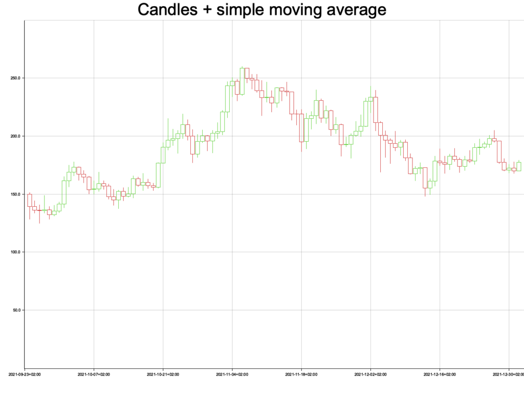
We now have a nice candlestick plot. As mentioned, the candlesticks are not filled with color. Hopefully, that will get fixed in a future version of the plotters crate.
Adding a Simple Moving Average (SMA) line
Next, we will add an SMA line graph on top of the candlesticks. As mentioned at the start we will use a function we wrote in an earlier tutorial to calculate the SMA. Please refer to that tutorial if you wish to learn more about the function.
SMA function summary
Let’s add the function to main.rs below the main() function:
pub fn simple_moving_average(data_set: &Vec<f64>, window_size: usize) -> Option<Vec<f64>> {
    if window_size > data_set.len() {
        return None;
    }

    let mut result: Vec<f64> = Vec::new();
    let mut window_start = 0;
    while window_start + window_size <= data_set.len() {
        let window_end = window_start + window_size;
        let data_slice = &data_set[window_start..window_end];
        let sum: f64 = data_slice.iter().sum();
        let average = sum / window_size as f64;
        result.push(average);
        window_start += 1;
    }

    Some(result)
}
The function takes a reference to a Vec<f64> and a window_size. The window size determines how many data points are used to calculate the average. The SMA data will be shorter in length than the input data because we need a number of items to fit the window size. So if we have a window size of 2 and data is [100, 150, 200, 300], the first set of data points is 100 and 150, then 150 and 200, and finally 200 and 300. We end up with [125, 175, 250] for the SMA data.
SMA line data preparation
We have to do some data transformations to first be able to calculate the SMA on our current data, and then transform that data into something plotters can work with.
First, calculating the SMA:
    let close_price_data: Vec<f64> = data.iter().map(|x| x.4 as f64).collect();
    let sma_data = simple_moving_average(&close_price_data, 15).expect("Calculating SMA failed");

    let mut line_data: Vec<(Date<Local>, f32)> = Vec::new();
    for i in 0..sma_data.len() {
        line_data.push((data[i].0, sma_data[i] as f32));
    }
On line 56 we take the “close price” from our data set and turn it into a Vec<f64> to be passed to the simple_moving_average function on line 57. We set a time window of 15, to calculate the Simple Moving Average on a period of 15 days in this case.
Then we have to prepare the data for the line graph so we have to add Date<Local> information. We do this on lines 59-62.
We now have everything in place to complete our “plot candles and SMA with Rust” project.
Drawing the SMA plot on the Candlesticks plot
To add another plot to the chart we just have to call .draw_series() again on the chart object. This time we will call it with a LineSeries object:
    chart
        .draw_series(LineSeries::new(line_data, BLUE.stroke_width(2)))
        .unwrap()
        .label("SMA 15")
        .legend(|(x, y)| PathElement::new(vec![(x, y), (x + 20, y)], &BLUE));
Here we simply pass the line_data value we create before and set the color with a “stroke-width” which is the thickness of the line. Then on line 67, we set a text for the legend and on line 68 we set a symbol. In this case, the symbol is a horizontal line 20 pixels long.
Finally, let’s draw the legend explaining what the SMA line is:
   chart
        .configure_series_labels()
        .position(SeriesLabelPosition::UpperMiddle)
        .label_font(("sans-serif", 30.0).into_font())
        .background_style(WHITE.filled())
        .draw()
        .unwrap();
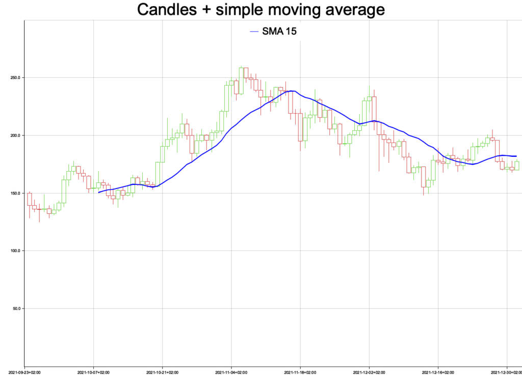
With these lines, we configure the position, font, font size, and background of the legend.
Running the program now should result in the following image:
Adding a second SMA line
Adding another SMA is very easy now, simply copy part of what we did in the previous section and put it between chart.draw_series and chart.configure_series_labels:
    let close_price_data: Vec<f64> = data.iter().map(|x| x.4 as f64).collect();
    let sma_data = simple_moving_average(&close_price_data, 15).expect("Calculating SMA failed");

    let mut line_data: Vec<(Date<Local>, f32)> = Vec::new();
    for i in 0..sma_data.len() {
        line_data.push((data[i].0, sma_data[i] as f32));
    }

    chart
        .draw_series(LineSeries::new(line_data, BLUE.stroke_width(2)))
        .unwrap()
        .label("SMA 15")
        .legend(|(x, y)| PathElement::new(vec![(x, y), (x + 20, y)], &BLUE));

    let sma_data = simple_moving_average(&close_price_data, 30).expect("Calculating SMA failed");

    let mut line_data: Vec<(Date<Local>, f32)> = Vec::new();
    for i in 0..sma_data.len() {
        line_data.push((data[i].0, sma_data[i] as f32));
    }

    chart
        .draw_series(LineSeries::new(
            line_data,
            RGBColor(150, 50, 168).stroke_width(2),
        ))
        .unwrap()
        .label("SMA 30")
        .legend(|(x, y)| PathElement::new(vec![(x, y), (x + 20, y)], &RGBColor(150, 50, 168)));

    chart
        .configure_series_labels()
        .position(SeriesLabelPosition::UpperMiddle)
        .label_font(("sans-serif", 30.0).into_font())
        .background_style(WHITE.filled())
        .draw()
        .unwrap();
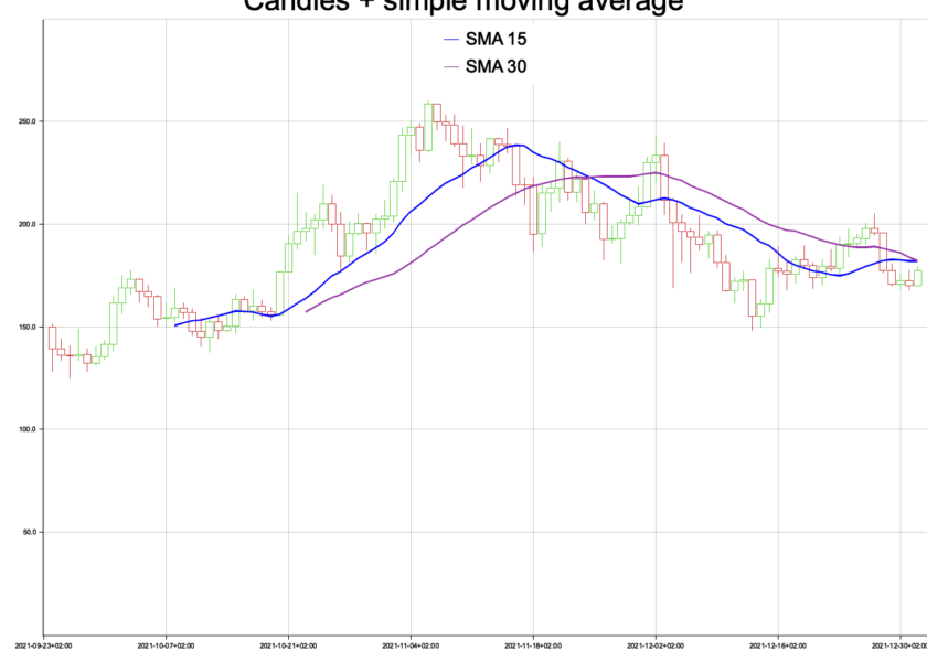
Now when we run the program we get the following result:
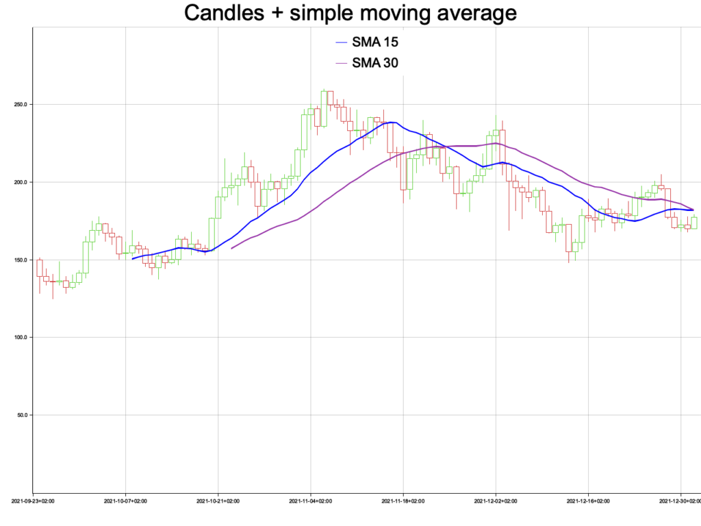
Conclusion
We have learned the basics of how to plot candles and the SMA indicator with Rust using plotters. Next to that, we learned a little bit about transforming and preparing data for our plot. In the end, we create a nice plot showing candles and two SMA lines with Rust for fictional price data.
In a future tutorial, we will look at how to draw other types of plots and other kinds of technical indicators.
The complete project code can be found on my GitHub: https://github.com/tmsdev82/rust-plotters-sma-tutorial.
Please follow me on Twitter to get notified on new Rust programming and technical indicator plotting related articles:
Follow @tmdev82
Hello sir, I like your articles. Did you think to put it all together into a working trading terminal? I think there is no cross platform terminal that offers snappy experience.